When I sat for the CFA exams, the syllabus pertaining to performance attribution was mostly written by the Brinson crowd – Brinson, Hood, Karnosky, Singer, et al. It was helpful to have a framework for clarifying how much return in a discrete time period was attributable to aspects such as security vs. sector selection, country vs. currency allocation, and active decisions vs. policy decisions.
That literature was pioneering because it clarified a subtlety about non-domestic returns that is not intuitively obvious, namely that total returns depend not merely on the the local return plus changes in foreign exchange rates, but also on the differences between domestic and local risk-free rates.
What the literature was silent on was how to link attributed results from one period to the next1. Due to the absence of a standard on this aspect, deriving how to link performance attribution over time became my first project after business school.
Applying a mindset I had learned in a Cost Accounting course, I arrived at a method that turns out to be similar to ones since identified by others (Carino, Frongello, Menchero). Namely: any discrete active contribution affects the total cumulative return to-date, and forever after it will earn the benchmark (or policy) return. It becomes a permanent part of the fund. While it can be offset by future active effects, the passing of time itself will not diminish or dilute the relative active effect once it’s been experienced.
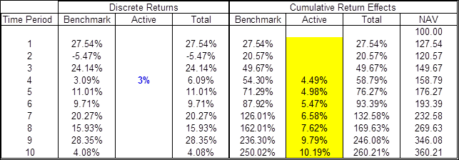
The image below shows a simple 10-period attribution, illustrated with an active effect only in period 4. Imagine a fund that doesn’t employ active managers, then employs one in Period 4, but then fires2 the active manager after that period.
In this example the active effect has nearly doubled the fund’s return for the 4th period. Notice, however that the cumulative effect is much greater than the discrete effect: that’s because the size of the fund is due to the fund’s cumulative historical return. At time zero the fund NAV was 100; by the end of period 4 the fund already had grown to a different NAV. The 3% contribution to the fund at this point increases the fund since-inception unit value not by 3% but by 4.49%, having been scaled up to reflect the prior cumulative return since-inception. Forevermore that effect lives on in the fund, and even though the active manager gets fired that contribution earns the benchmark return, for better or worse.
Clearly this is a sanguine example, and an unlikely one in which the active manager would be terminated after a positive contribution. So play with your own data – here is a spreadsheet you can play with and try different active contributions in different periods to witness the effects. Be aware that the Benchmark returns are randomly generated, so when you play with the spreadsheet they will change unless you download the sheet to Excel.
1Eventually I discussed the topic of linked attribution with one of these authors and was disappointed that he dismissed the matter of linking attribution results as trivial compared to the attribution framework itself. For the purpose of performance attribution I concede the point, but comprehending the intuition of linking attribution has been crucial ever since for grasping how alpha and beta work and impact performance over time, and also for appreciating why not every anomaly is exploitable.
2Pardon the digression, but if you think it’s implausible that a fund would fire active managers after beating their benchmark so handsomely, all I will say is liquidity needs make for curious decisions. There was some bizarre stuff going on during and after the financial crisis. I’ll leave it at that.
